AIR POLLUTION USING R
On this page you are able to see how did I analised the pollution of Manresa and the wind of Badalona, since 2013 and 2014, to 2021. This project is made with R language.
1. Data collection
Here you have the webs where it can be found all the data:
-We must take into account that the data are hourly for pollution and the meteorological data are semi-hourly (every 30 minutes) that we have to combine in a single dataframe to make graphs that relate both types of data. The weather data will be from the station closest to our pollution station.
-From the meteorological data the codes of the variables that we need are 30 for wind speed that we will put ws, and 31 for wind direction that we will put wd. The dates will be in ISO8601 format 2021-03-15 16:00:00 with POSIXct format with the name date. The names date, ws and wd are Openair requirements.
2. Required software
The program needed is RStudio and its packages tidyverse i openair. Tidyverse is used to tidy the data, as it's said on its name. And Openair allows hour by hour, day by day, year by year air studies in a specific and advanced way. In order to install both packages you just have to type:
install.packages (c("tidyverse","openair"))3. Tidying the atmospheric data
We must read the data from our computer:
city<-read.csv("C://Users/YOURCOMPUTERNAME/Documents/city.csv")View(city)We change the times of the columns to rows:
city1<-pivot_longer(city,cols=c(h01,h02,h03,h04,h05,h06,h07,h08,h09,h10,h11,h12,h13,h14, h15,h16,h17,h18,h19,h20,h21,h22,h23,h24), names_to="hour", values_to = "value")4. Modifying the atmospheric data with Visual Studio Code
We delete the useless data and we export the project into our computer:
city2<-city1[-c(1,2,4,6:16)]write.csv(city2,"C:\\Users\\YOURCOMPUTERNAME\\Documents\\city2.csv")We delete T00.00.00.000 and replace the times H01, etc for 01:00:00 until we get the dates in ISO format:
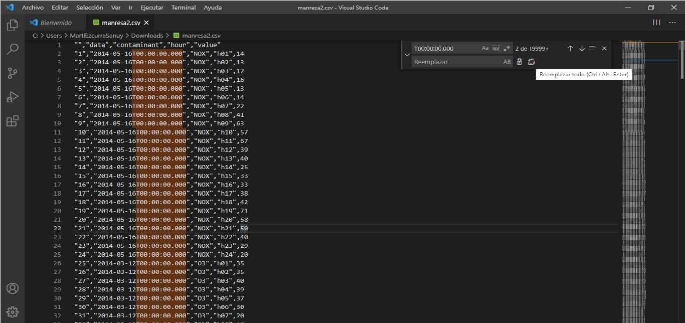
We associate date and time together to city4.csv using LibreOffice Calc or RStudio.
city4 <- city3 %>% mutate(name=paste0(data, " ", hour))We create city5 by putting day and time together under the column name date:
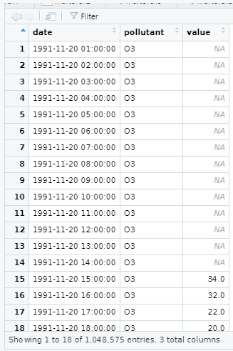
5. Convert data format
library(openair)city5NO2 <- subset(city5, pollutant=="NO2")city5NO2$date<-as.POSIXct(city5NO2$date,"%Y-%m-%d %H:%M:%S", tz="Europe/Madrid")class(city5NO2$date)[1] "POSIXct" "POSIXt"View(city5NO2)We must be careful, it has to be a POSIXct(a date), instead of characters:
city5NO2$date<-as.POSIXct(city5NO2$date,"%Y-%m-%d %H:%M:%S", tz="Europe/Madrid")
class(city5NO2$date)
[1] "POSIXct" "POSIXt"
6. Creating graphics with Openair R
timeVariation(city5NO2, pollutant="value")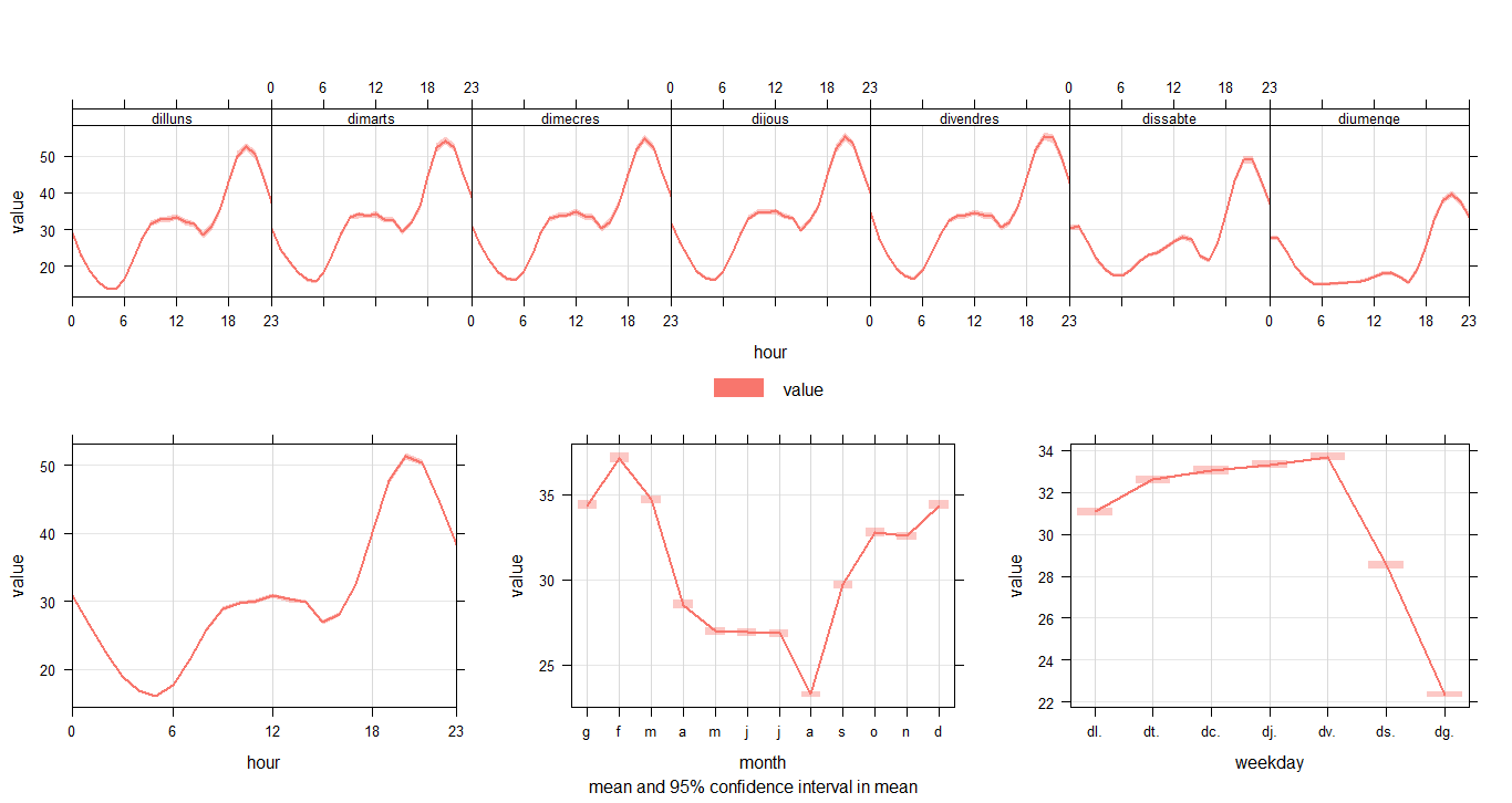
trendLevel(city5NO2, pollutant = "value", main="Hydrogen sulfide evolution in MYCITYNAME")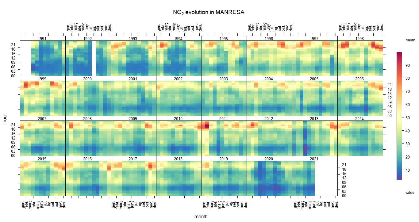
daily<-timeAverage(city5NO2,avg.time = "day")View(daily) calendarPlot(city%NO2, pollutant="value", year="2020")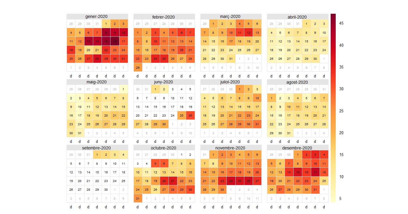
yearly<-timeAverage(city5no2,avg.time = "year")View(yearly)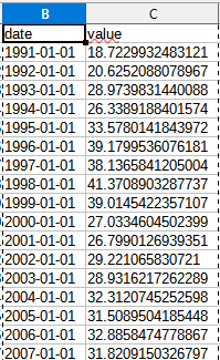
timePlot(selectByDate(city6), pollutant = c("NOX","NO2","CO","SO2","H2S","NO","PM10","O3", "HCT","HCNM"), y.relation = "free", main="Yearly mean of air pollutants in MYCITYNAME")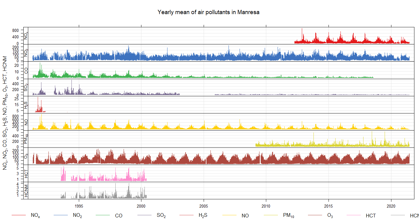
7. Sorting data with pivot_wider
library(tidyverse)city6<-pivot_wider(city5, names_from= pollutant, values_from =value)View (city6)write.csv(city6,"C:\\Users\\ELMEUNOM\\Documents\\LAMEVACIUTAT\\city6.csv")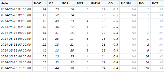
8. Temporary variation of pollutants 2013-2021
city6$date<- as.POSIXct(city6$date,format="%Y-%m-%d %H:%M:%S",tz="Europe/Madrid")timeVariation(city6, pollutant=c("O3","NO2","H2S","NO","HCNM","CO","SO2","HCT", "NOX","PM10"), main="Air pollution in MYCITYNAME (1991-2021)")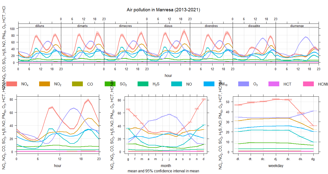
9. Sorting weather data
wind<-read.csv("C://Users/YOURCOMPUTERNAME/Documents/wind.csv")View(wind)wind1←wind[-c(1,2,5,7,8)]wind2<-pivot_wider(wind1,names_from = CODI_VARIABLE, values_from = VALOR_LECTURA)names(wind2)[names(wind2) == "31"] <- "wd"names(wind2)[names(wind2) == "30"] <- "ws"names(wind2)[names(wind2) == "DATA_LECTURA"] <- "date"write.csv(wind2,"C:\\Users\\YOURCOMPUTERNAME\\Documents\\wind2.csv")wind3<-timeAverage(wind2, time.avg="hour")cityall<-merge(city6, wind6, by ="date")View (cityall)
10. PollutionRose
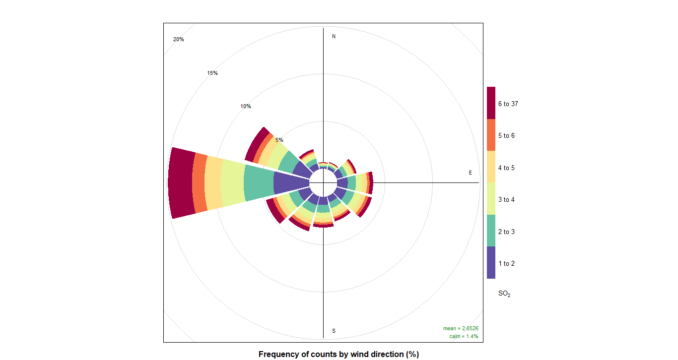
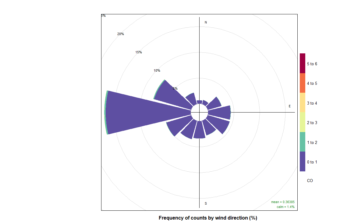
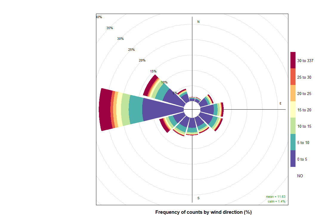
And now we can do pollutionRose and see where the pollution is coming from wwith that instruction:
pollutionRose(cityall, pollutant = "contaminant")CO:
NO:
NO2
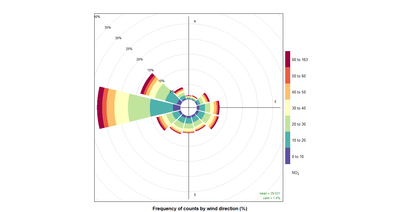
NOX:
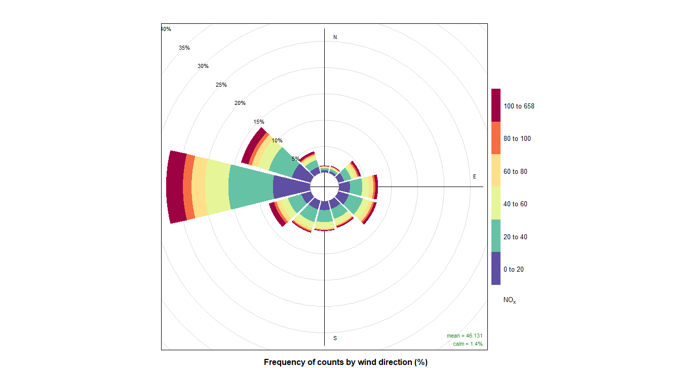
O3:
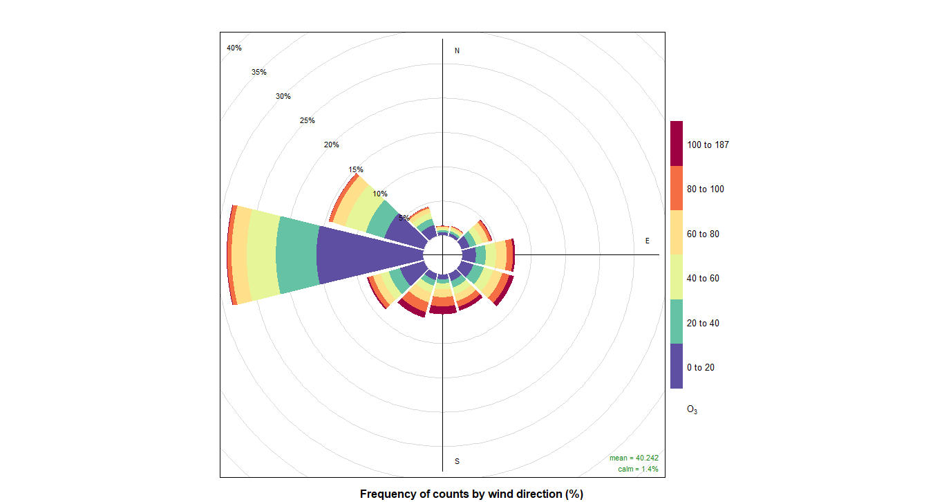
PM10
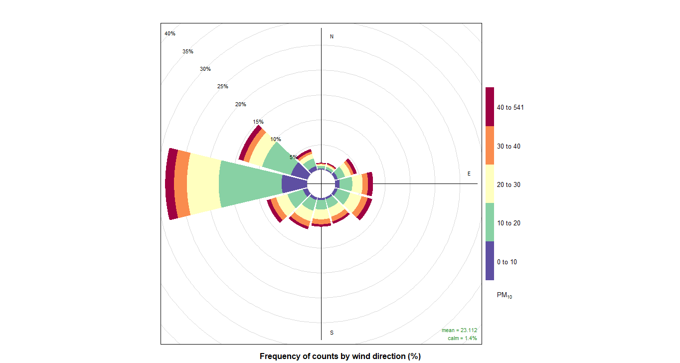
SO2
